The above distribution is discontinuous converting into continuous distribution, we get :
Adjustment factor = (Lower limit of one class - Upper limit of previous class) / 2
= $\frac{20 - 19}{2} = \frac{1}{2}$
= 0.5
Subtract the adjustment factor (0.5) from all the lower limits and add the adjustment factor (0.5) to all the upper limits.
| Classes before adjustment | Classes after adjustment | Frequency | Cumulative frequency |
|---|
| 10 - 19 | 9.5 - 19.5 | 23 | 23 |
| 20 - 29 | 19.5 - 29.5 | 16 | 39 (23 + 16) |
| 30 - 39 | 29.5 - 39.5 | 15 | 54 (39 + 15) |
| 40 - 49 | 39.5 - 49.5 | 20 | 74 (54 + 20) |
| 50 - 59 | 49.5 - 59.5 | 12 | 86 (74 + 12) |
Steps of construction of ogive :
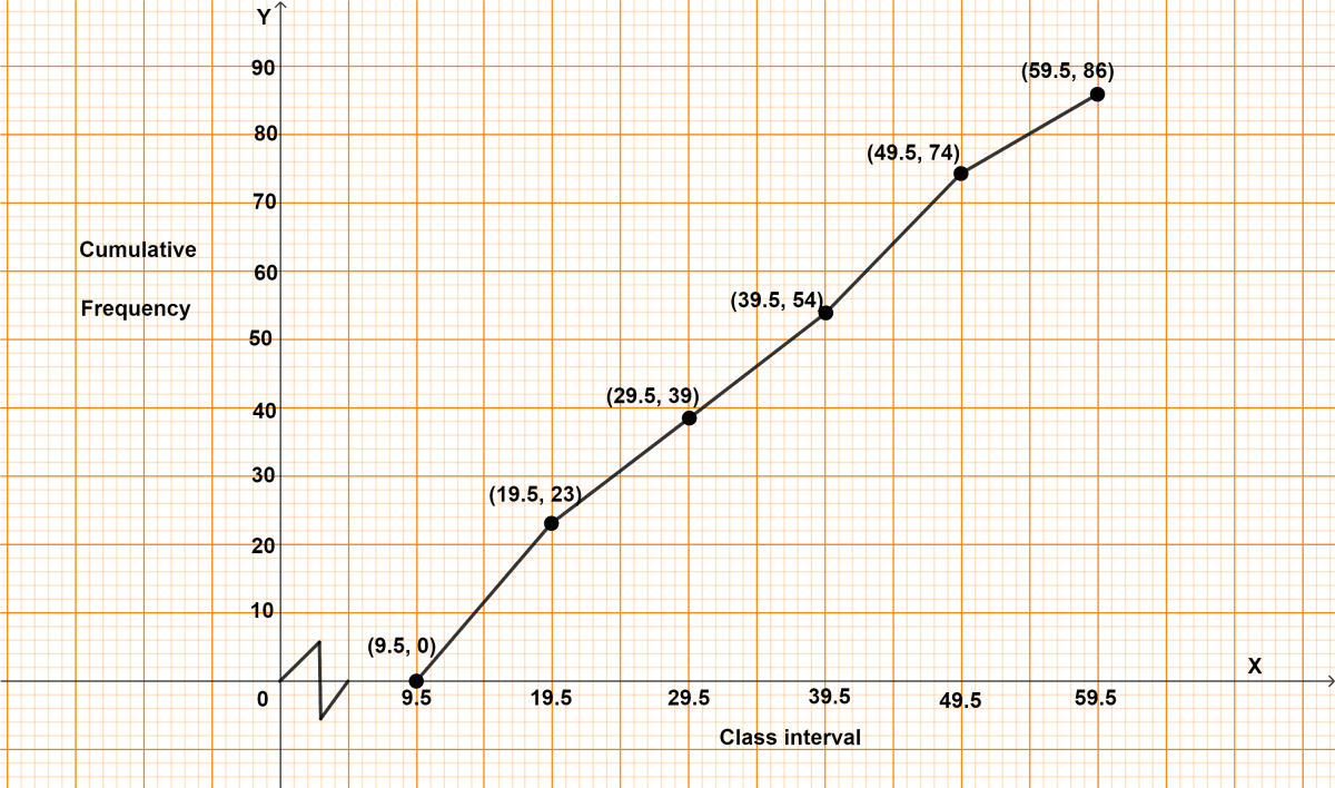
Since, the scale on x-axis starts at 9.5, a break (kink) is shown near the origin on x-axis to indicate that the graph is drawn to scale beginning at 9.5.
Take 2 cm = 10 units along x-axis.
Take 1 cm = 10 units along y-axis.
Ogive always starts from a point on x-axis representing the lower limit of the first class. Mark point (9.5, 0).
Take upper class limits along x-axis and corresponding cumulative frequencies along y-axis, mark the points (19.5, 23), (29.5, 39), (39.5, 54), (49.5, 74) and (59.5, 86).
Join the points marked by a free hand curve.
The required ogive is shown in the below figure: